Scaling CMA-MAE on the Sphere Benchmark
![]()
This tutorial is part of the series of pyribs tutorials! See here for the list of all tutorials and the order in which they should be read.
One challenge in applying CMA-MAE is its quadratic time complexity. Internally, CMA-MAE relies on CMA-ES, which has \(\Theta(n^2)\) time and space complexity due to operations on an \(n \times n\) covariance matrix. Thus, CMA-ES and hence CMA-MAE can be computationally intractable when a problem involves millions or even just thousands of parameters. To address this issue, Tjanaka 2023 proposes to replace CMA-ES with more efficient evolution strategies (ESs), resulting in several variants of CMA-MAE. The CMA-MAE variants proposed in the paper and supported in pyribs are as follows:
LM-MA-MAE: Replaces CMA-ES with Limited Memory Matrix Adaptation ES (LM-MA-ES), which has \(\Theta(kn)\) runtime.
sep-CMA-MAE: Replaces CMA-ES with separable CMA-ES (sep-CMA-ES), which constrains the covariance matrix to be diagonal and has \(\Theta(n)\) runtime.
OpenAI-MAE: Replaces CMA-ES with OpenAI-ES, which performs search by sampling from an isotropic Gaussian and has \(\Theta(n)\) runtime.
This tutorial shows how these different variants of CMA-MAE can be accessed by changing the es parameter in the EvolutionStrategyEmitter.
Note: This tutorial is based on the CMA-MAE tutorial. As such, we skim over details like how to set up the archives. For more details on these steps, please refer to that tutorial.
Setup
%pip install ribs[visualize] tqdm
import sys

import matplotlib.pyplot as plt
import numpy as np
from tqdm import tqdm, trange
The Sphere Linear Projection Benchmark
In this tutorial, we use a 1000-dimensional version of the sphere benchmark. At this dimensionality, CMA-MAE becomes extremely slow due to its quadratic complexity.
def sphere(solutions: np.ndarray) -> tuple[np.ndarray, np.ndarray]:
    """Sphere function evaluation and measures for a batch of solutions.

    Args:
        solutions: (batch_size, dim) batch of solutions.

    Returns:
        objectives: (batch_size,) batch of objectives.
        measures: (batch_size, 2) batch of measures.
    """
    dim = solutions.shape[1]

    # Shift the Sphere function so that the optimal value is at x_i = 2.048.
    sphere_shift = 5.12 * 0.4

    # Normalize the objective to the range [0, 100] where 100 is optimal.
    best_obj = 0.0
    worst_obj = (-5.12 - sphere_shift) ** 2 * dim
    raw_obj = np.sum(np.square(solutions - sphere_shift), axis=1)
    objectives = (raw_obj - worst_obj) / (best_obj - worst_obj) * 100

    # Calculate measures.
    clipped = solutions.copy()
    clip_mask = (clipped < -5.12) | (clipped > 5.12)
    clipped[clip_mask] = 5.12 / clipped[clip_mask]
    measures = np.concatenate(
        (
            np.sum(clipped[:, : dim // 2], axis=1, keepdims=True),
            np.sum(clipped[:, dim // 2 :], axis=1, keepdims=True),
        ),
        axis=1,
    )

    return objectives, measures
Archive Setup
Note this archive has higher resolution (250x250) than the one in the CMA-MAE tutorial (100x100). As described in Appendix K of the CMA-MAE paper, this is necessary due to the high dimensionality of the domain.
from ribs.archives import GridArchive

max_bound = 1000 / 2 * 5.12

archive = GridArchive(
    solution_dim=1000,
    dims=(250, 250),
    ranges=[(-max_bound, max_bound), (-max_bound, max_bound)],
    learning_rate=0.01,
    threshold_min=0.0,
)

result_archive = GridArchive(
    solution_dim=1000,
    dims=(250, 250),
    ranges=[(-max_bound, max_bound), (-max_bound, max_bound)],
)
Emitter Setup with the es Parameter
Exactly like in the regular CMA-MAE, scalable variants of CMA-MAE are built with the EvolutionStrategyEmitter. The key difference is the choice of ES, which is indicated with the es parameter. es has the following options:
lm_ma_es: Indicates LM-MA-ESsep_cma_es: Indicates sep-CMA-ESopenai_es: Indicates OpenAI-ES
Below, we first show how to use sep_cma_es by passing es="sep_cma_es".
from ribs.emitters import EvolutionStrategyEmitter

emitters = [
    EvolutionStrategyEmitter(
        archive,
        x0=np.zeros(1000),
        sigma0=0.5,
        ranker="imp",
        es="sep_cma_es",
        selection_rule="mu",
        restart_rule="basic",
        batch_size=36,
    )
    for _ in range(15)
]
It is also possible to pass in es as a class, as the string options to es are simply translated to a corresponding ES class (the documentation for all ES classes is here). All ES classes are subclasses of EvolutionStrategyBase.
from ribs.emitters.opt import SeparableCMAEvolutionStrategy

emitters_v2 = [
    EvolutionStrategyEmitter(
        archive,
        x0=np.zeros(1000),
        sigma0=0.5,
        ranker="imp",
        es=SeparableCMAEvolutionStrategy,
        selection_rule="mu",
        restart_rule="basic",
        batch_size=36,
    )
    for _ in range(15)
]
Some ESs also accept kwargs. For instance, in LMMAEvolutionStrategy, the size of the approximation can be adjusted with the n_vectors parameter. kwargs can be passed to the ESs with the es_kwargs parameter in EvolutionStrategyEmitter, as shown below.
# Regular instantiation of EvolutionStrategyEmitter with `lm_ma_es`.
lm_ma_emitters = [
    EvolutionStrategyEmitter(
        archive,
        x0=np.zeros(1000),
        sigma0=0.5,
        ranker="imp",
        es="lm_ma_es",
        selection_rule="mu",
        restart_rule="basic",
        batch_size=36,
    )
    for _ in range(15)
]

# Instantiation of EvolutionStrategyEmitter with `lm_ma_es` and kwargs.
lm_ma_emitters_v2 = [
    EvolutionStrategyEmitter(
        archive,
        x0=np.zeros(1000),
        sigma0=0.5,
        ranker="imp",
        es="lm_ma_es",
        es_kwargs={"n_vectors": 20},
        selection_rule="mu",
        restart_rule="basic",
        batch_size=36,
    )
    for _ in range(15)
]
Finally, GradientArborescenceEmitter also has as es parameter. However, it is less common to use a scalable ES in GradientArborescenceEmitter since the ES only operates in objective-measure coefficient space, and that space usually has only a few dimensions.
Scheduler Setup
Note that we only use the emitters created above with es="sep_cma_es".
from ribs.schedulers import Scheduler

scheduler = Scheduler(archive, emitters, result_archive)
Running Scalable CMA-MAE
Finally, we run the scalable CMA-MAE variant created above on a 1000-dimensional sphere function.
total_itrs = 10_000

for itr in trange(1, total_itrs + 1, file=sys.stdout, desc="Iterations"):
    solutions = scheduler.ask()
    objectives, measures = sphere(solutions)
    scheduler.tell(objectives, measures)

    # Output progress every 500 iterations or on the final iteration.
    if itr % 500 == 0 or itr == total_itrs:
        tqdm.write(
            f"Iteration {itr:5d} | "
            f"Archive Coverage: {result_archive.stats.coverage:6.3%}  "
            f"Normalized QD Score: {result_archive.stats.norm_qd_score:6.3f}"
        )
Iteration   500 | Archive Coverage:  7.370%  Normalized QD Score:  6.729
Iteration  1000 | Archive Coverage: 12.394%  Normalized QD Score: 10.728
Iteration  1500 | Archive Coverage: 15.531%  Normalized QD Score: 13.100
Iteration  2000 | Archive Coverage: 17.366%  Normalized QD Score: 14.356
Iteration  2500 | Archive Coverage: 19.149%  Normalized QD Score: 15.670
Iteration  3000 | Archive Coverage: 19.944%  Normalized QD Score: 16.195
Iteration  3500 | Archive Coverage: 21.136%  Normalized QD Score: 17.101
Iteration  4000 | Archive Coverage: 22.966%  Normalized QD Score: 18.396
Iteration  4500 | Archive Coverage: 24.563%  Normalized QD Score: 19.464
Iteration  5000 | Archive Coverage: 25.526%  Normalized QD Score: 20.108
Iteration  5500 | Archive Coverage: 26.158%  Normalized QD Score: 20.590
Iteration  6000 | Archive Coverage: 26.355%  Normalized QD Score: 20.834
Iteration  6500 | Archive Coverage: 26.579%  Normalized QD Score: 21.059
Iteration  7000 | Archive Coverage: 26.579%  Normalized QD Score: 21.132
Iteration  7500 | Archive Coverage: 26.667%  Normalized QD Score: 21.257
Iteration  8000 | Archive Coverage: 26.667%  Normalized QD Score: 21.340
Iteration  8500 | Archive Coverage: 26.667%  Normalized QD Score: 21.377
Iteration  9000 | Archive Coverage: 26.667%  Normalized QD Score: 21.441
Iteration  9500 | Archive Coverage: 26.667%  Normalized QD Score: 21.455
Iteration 10000 | Archive Coverage: 26.667%  Normalized QD Score: 21.479
Iterations: 100%|███████████████████████████████████████| 10000/10000 [03:30<00:00, 47.41it/s]
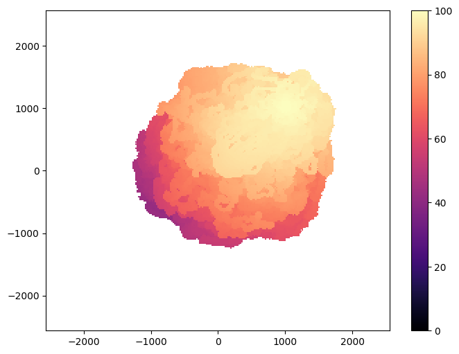
Visualization
from ribs.visualize import grid_archive_heatmap

plt.figure(figsize=(8, 6))
grid_archive_heatmap(result_archive, vmin=0, vmax=100)
Citation
If you find this tutorial useful, please cite it as:
@article{pyribs_scalable_cma_mae,
  title   = {Scaling CMA-MAE on the Sphere Benchmark},
  author  = {Henry Chen and Bryon Tjanaka and Stefanos Nikolaidis},
  journal = {pyribs.org},
  year    = {2023},
  url     = {https://docs.pyribs.org/en/stable/tutorials/cma_mae.html}
}