Illuminating the Latent Space of an MNIST GAN
![]()
This tutorial is part of the series of pyribs tutorials! See here for the list of all tutorials and the order in which they should be read.
One of the most popular applications of Generative Adversarial Networks is generating fake images. In particular, websites like this person does not exist serve a GAN that generates fake images of people (this x does not exist provides a comprehensive list of such websites). Such websites are entertaining, especially when one is asked to figure out which face is real.
Usually, these websites extract fake images by sampling the GAN’s latent space. For those unfamiliar with GANs, this means that each image is associated with a real valued vector of \(n\) components. But since these vectors are typically generated randomly, the usefulness of these websites breaks down when we wish to search for a specific image.
For instance, suppose that instead of fake faces, we want to generate fake handwriting, specifically the digit eight (8). We could train a GAN on the MNIST dataset and produce a generator network that generates fake digits. Now, we can repeatedly sample the latent space until an eight appears. However, if we want to find an eight, we could optimize latent space directly with CMA-ES. To ensure that we generate eights, we could use the output classification prediction of a LeNet-5 classifier as the objective (see Bontrager 2018).1 But notice that the latent space likely contains many examples of the digit eight, and they might vary in the weight of the pen stroke or the lightness of the ink color. If we make these properties our measures, we could search latent space for many different examples of eight in a single run!
Fontaine 2021 takes exactly this approach when generating new levels for the classic video game Super Mario Bros. They term this approach “Latent Space Illumination”, as they explore quality diversity (QD) algorithms (including CMA-ME) as a method to search the latent space of a video game level GAN and illuminate the space of possible level mechanics. In this tutorial, we illuminate the latent space of the aforementioned MNIST GAN by mimicking the approach taken in Fontaine 2021.
1Since the discriminator of the GAN is only trained to evaluate how realistic an image is, it cannot detect specific digits. Hence, we need the LeNet-5 to check that the digit is an 8.
Setup
First, we install pyribs, PyTorch, and several utilities.
%pip install ribs[visualize] torch torchvision numpy matplotlib tqdm
import sys

import matplotlib.pyplot as plt
import numpy as np
import torch
from torch import nn
from tqdm import tqdm, trange
Below, we check what device is available for PyTorch. On Colab, activate the GPU by clicking “Runtime” in the toolbar at the top. Then, click “Change Runtime Type”, and select “GPU”.
device = torch.device("cuda" if torch.cuda.is_available() else "cpu")
print(device)
Loading the GAN and Classifier
For this tutorial, we pretrained a GAN that generates MNIST digits using the code from a beginner GAN tutorial. We also pretrained a LeNet-5 classifier for the MNIST dataset using the code here. Below, we define the network structures.
class Generator(nn.Module):
    """Generator network for the GAN."""

    def __init__(self, nz: int) -> None:
        super().__init__()

        # Size of the latent space (number of dimensions).
        self.nz = nz
        self.main = nn.Sequential(
            nn.Linear(self.nz, 256),
            nn.LeakyReLU(0.2),
            nn.Linear(256, 512),
            nn.LeakyReLU(0.2),
            nn.Linear(512, 1024),
            nn.LeakyReLU(0.2),
            nn.Linear(1024, 784),
            nn.Tanh(),
        )

    def forward(self, x: torch.Tensor) -> torch.Tensor:
        return self.main(x).view(-1, 1, 28, 28)


class Discriminator(nn.Module):
    """Discriminator network for the GAN."""

    def __init__(self) -> None:
        super().__init__()
        self.n_input = 784
        self.main = nn.Sequential(
            nn.Linear(self.n_input, 1024),
            nn.LeakyReLU(0.2),
            nn.Dropout(0.3),
            nn.Linear(1024, 512),
            nn.LeakyReLU(0.2),
            nn.Dropout(0.3),
            nn.Linear(512, 256),
            nn.LeakyReLU(0.2),
            nn.Dropout(0.3),
            nn.Linear(256, 1),
            nn.Sigmoid(),
        )

    def forward(self, x: torch.Tensor) -> torch.Tensor:
        x = x.view(-1, 784)
        return self.main(x)


LENET5 = nn.Sequential(
    nn.Conv2d(1, 6, (5, 5), stride=1, padding=0),  # (1,28,28) -> (6,24,24)
    nn.MaxPool2d(2),  # (6,24,24) -> (6,12,12)
    nn.ReLU(),
    nn.Conv2d(6, 16, (5, 5), stride=1, padding=0),  # (6,12,12) -> (16,8,8)
    nn.MaxPool2d(2),  # (16,8,8) -> (16,4,4)
    nn.ReLU(),
    nn.Flatten(),  # (16,4,4) -> (256,)
    nn.Linear(256, 120),  # (256,) -> (120,)
    nn.ReLU(),
    nn.Linear(120, 84),  # (120,) -> (84,)
    nn.ReLU(),
    nn.Linear(84, 10),  # (84,) -> (10,)
    nn.LogSoftmax(dim=1),  # (10,) log probabilities
).to(device)
LENET5_MEAN_TRANSFORM = 0.1307
LENET5_STD_DEV_TRANSFORM = 0.3081
Next, we load the pretrained weights for each network.
from pathlib import Path
from urllib.request import urlretrieve

LOCAL_DIR = Path("lsi_mnist_weights")
LOCAL_DIR.mkdir(exist_ok=True)
WEB_DIR = "https://raw.githubusercontent.com/icaros-usc/pyribs/master/tutorials/mnist/"

# Download the model files to LOCAL_DIR.
for filename in [
    "mnist_generator.pth",
    "mnist_discriminator.pth",
    "mnist_classifier.pth",
]:
    model_path = LOCAL_DIR / filename
    if not model_path.is_file():
        urlretrieve(WEB_DIR + filename, str(model_path))

# Load the weights of each network from its file.
g_state_dict = torch.load(
    str(LOCAL_DIR / "mnist_generator.pth"),
    map_location=device,
)
d_state_dict = torch.load(
    str(LOCAL_DIR / "mnist_discriminator.pth"),
    map_location=device,
)
c_state_dict = torch.load(
    str(LOCAL_DIR / "mnist_classifier.pth"),
    map_location=device,
)

# Instantiate networks and insert the weights.
generator = Generator(nz=128).to(device)
discriminator = Discriminator().to(device)
generator.load_state_dict(g_state_dict)
discriminator.load_state_dict(d_state_dict)
LENET5.load_state_dict(c_state_dict)
<All keys matched successfully>
LSI with CMA-ME on MNIST GAN
After loading the GAN and the classifier, we can begin exploring the latent space of the GAN with the pyribs implementation of CMA-ME. Thus, we import and initialize the GridArchive, EvolutionStrategyEmitter, and Scheduler from pyribs.
For the GridArchive, we choose a 2D measure space with “boldness” and “lightness” as the measures. We approximate “boldness” of a digit by counting the number of white pixels in the image, and we approximate “lightness” by averaging the values of the white pixels in the image. We define a “white” pixel as a pixel with value at least 0.5 (pixels are bounded to the range \([0,1]\)). Since there are 784 pixels in an image, boldness is bounded to the range \([0, 784]\). Meanwhile, lightness is bounded to the range \([0.5, 1]\), as that is the range of a white pixel.
from ribs.archives import GridArchive

archive = GridArchive(
    solution_dim=generator.nz,
    dims=[200, 200],  # 200 cells along each dimension.
    ranges=[(0, 784), (0.5, 1)],  # Boldness range, lightness range.
)
Next, we use 5 instances of EvolutionStrategyEmitter with two-stage improvement ranking (“2imp”), each with batch size of 30. Each emitter begins with a zero vector of the same dimensionality as the latent space and an initial step size \(\sigma=0.2\).
from ribs.emitters import EvolutionStrategyEmitter

emitters = [
    EvolutionStrategyEmitter(
        archive=archive,
        x0=np.zeros(generator.nz),
        sigma0=0.2,  # Initial step size.
        ranker="2imp",
        batch_size=30,
    )
    for _ in range(5)  # Create 5 separate emitters.
]
Finally, we construct the scheduler to connect the archive and emitters together.
from ribs.schedulers import Scheduler

scheduler = Scheduler(archive, emitters)
With the components created, we now generate latent vectors. As we use 5 emitters with batch size of 30 and run 30,000 iterations, we evaluate 30,000 * 30 * 5 = 4,500,000 latent vectors in total. This loop will take anywhere between 5-30 min to run.
total_itrs = 30_000

for itr in trange(1, total_itrs + 1, file=sys.stdout, desc="Iterations"):
    solutions = scheduler.ask()

    with torch.no_grad():
        tensor_sols = torch.tensor(
            solutions,
            dtype=torch.float32,
            device=device,
        )

        # Shape: len(solutions) x 1 x 28 x 28
        generated_imgs = generator(tensor_sols)

        # Normalize the images from [-1,1] to [0,1].
        normalized_imgs = (generated_imgs + 1.0) / 2.0

        # We optimize the score of the digit being 8. Other digits may also be
        # used.
        lenet5_normalized = (
            normalized_imgs - LENET5_MEAN_TRANSFORM
        ) / LENET5_STD_DEV_TRANSFORM
        objectives = torch.exp(LENET5(lenet5_normalized)[:, 8]).cpu().numpy()

        # Shape: len(solutions) x 784
        flattened_imgs = (
            normalized_imgs.cpu().numpy().reshape((normalized_imgs.shape[0], -1))
        )

        # The first measures is the "boldness" of the digit (i.e. number of white
        # pixels). We consider pixels with values larger than or equal to 0.5
        # to be "white".
        # Shape: len(solutions) x 1
        boldness = np.count_nonzero(flattened_imgs >= 0.5, axis=1, keepdims=True)

        # The second measures is the "lightness" of the digit (i.e. the mean value of
        # the white pixels).
        # Shape: len(solutions) x 1
        flattened_imgs[flattened_imgs < 0.5] = 0  # Set non-white pixels to 0.
        # Add 1 to avoid dividing by zero.
        lightness = np.sum(flattened_imgs, axis=1, keepdims=True) / (boldness + 1)

        # Each measures entry is [boldness, lightness].
        measures = np.concatenate([boldness, lightness], axis=1)

    scheduler.tell(objectives, measures)

    if itr % 1000 == 0 or itr == total_itrs:
        tqdm.write(f"Iteration {itr} archive size: {len(archive)}")
Iteration 1000 archive size: 15189
Iteration 2000 archive size: 18422
Iteration 3000 archive size: 18784
Iteration 4000 archive size: 18936
Iteration 5000 archive size: 19202
Iteration 6000 archive size: 19321
Iteration 7000 archive size: 19373
Iteration 8000 archive size: 19775
Iteration 9000 archive size: 20835
Iteration 10000 archive size: 20865
Iteration 11000 archive size: 20877
Iteration 12000 archive size: 20908
Iteration 13000 archive size: 20936
Iteration 14000 archive size: 20968
Iteration 15000 archive size: 20998
Iteration 16000 archive size: 21034
Iteration 17000 archive size: 21050
Iteration 18000 archive size: 21110
Iteration 19000 archive size: 21130
Iteration 20000 archive size: 21141
Iteration 21000 archive size: 21161
Iteration 22000 archive size: 21179
Iteration 23000 archive size: 21187
Iteration 24000 archive size: 21198
Iteration 25000 archive size: 21211
Iteration 26000 archive size: 21227
Iteration 27000 archive size: 21250
Iteration 28000 archive size: 21253
Iteration 29000 archive size: 21258
Iteration 30000 archive size: 21264
Iterations: 100%|████████████████████████████████████████████████████████████████████████████████████████████████████| 30000/30000 [04:30<00:00, 111.06it/s]
from torchvision.utils import make_grid


def show_grid_img(
    x_start: int,
    x_num: int,
    x_step_size: int,
    y_start: int,
    y_num: int,
    y_step_size: int,
    archive: GridArchive,
    figsize: tuple[int, int] = (8, 6),
) -> None:
    """Displays a grid of images from the archive.

    Args:
        x_start: Starting index along x-axis.
        x_num: Number of images to generate along x-axis.
        x_step_size: Index step size along x-axis.
        y_start: Starting index along y-axis.
        y_num: Number of images to generate along y-axis.
        y_step_size: Index step size along y-axis.
        archive: Archive with results from CMA-ME.
        figsize: Size of the figure for the image.
    """
    x_range = np.arange(x_start, x_start + x_step_size * x_num, x_step_size)
    y_range = np.arange(y_start, y_start + y_step_size * y_num, y_step_size)
    grid_indices = [(x, y) for y in np.flip(y_range) for x in x_range]
    imgs = []
    img_size = (28, 28)
    solutions = archive.data("solution")
    indices = archive.data("index")
    int_indices = archive.grid_to_int_index(grid_indices)

    for int_index in int_indices:
        if not np.any(indices == int_index):
            print(f"There is no solution at index {int_index}.")
            return
        else:
            sol = solutions[indices == int_index]

        with torch.no_grad():
            img = generator(
                torch.tensor(
                    sol.reshape(1, generator.nz), dtype=torch.float32, device=device
                )
            )
            # Normalize images to [0,1].
            normalized = (img.reshape(1, *img_size) + 1) / 2
            imgs.append(normalized)

    plt.figure(figsize=figsize)
    img_grid = make_grid(imgs, nrow=x_num, padding=0)
    plt.imshow(
        np.transpose(img_grid.cpu().numpy(), (1, 2, 0)),
        interpolation="nearest",
        cmap="gray",
    )

    # Change labels to be measures.
    plt.xlabel("Boldness")
    plt.ylabel("Lightness")
    x_ticklabels = [
        round(archive.boundaries[0][i])
        for i in [x_start + x_step_size * k for k in range(x_num + 1)]
    ]
    y_ticklabels = [
        round(archive.boundaries[1][i], 2)
        for i in [
            y_start + y_step_size * y_num - y_step_size * k for k in range(y_num + 1)
        ]
    ]
    plt.xticks([img_size[0] * x for x in range(x_num + 1)], x_ticklabels)
    plt.yticks([img_size[0] * x for x in range(y_num + 1)], y_ticklabels)
Visualization
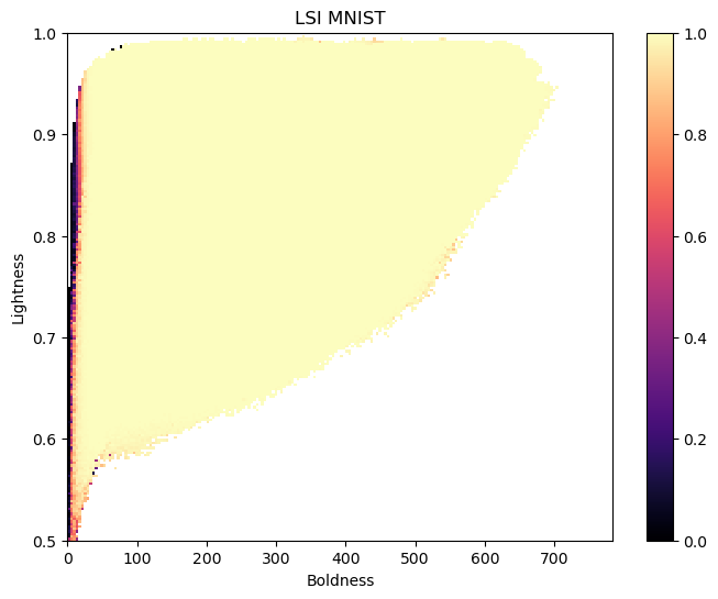
Below, we visualize the archive after all evaluations. The x-axis is the boldness and the y-axis is the lightness. The color indicates the objective value. We can see that we found many images that the classifier strongly believed to be an eight.
from ribs.visualize import grid_archive_heatmap

plt.figure(figsize=(8, 6))
grid_archive_heatmap(archive, vmin=0.0, vmax=1.0)
plt.title("LSI MNIST")
plt.xlabel("Boldness")
plt.ylabel("Lightness")
plt.show()
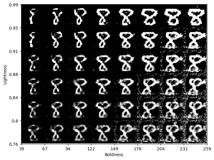
Next, we display a grid of digits generated from a selected set of latent vectors in the archive.
As we can see below, digits get bolder as we go along the x-axis. Meanwhile, as we go along the y-axis, the digits get brighter. For instance, the image in the bottom right corner is grey and bold, while the image in the top left corner is white and thin.
show_grid_img(10, 8, 7, 105, 6, 15, archive)
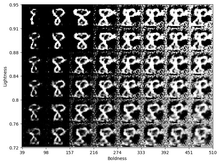
Here we display images from a wider range of the archive. Note that in order to generate images with high boldness values, CMA-ME generated images that do not look realistic (see the bottom right corner in particular).
show_grid_img(10, 8, 15, 90, 6, 15, archive)
To determine how realistic all of the images in the archive are, we can evaluate them with the discriminator network of the GAN. Below, we create a new archive where the objective value of each solution is the discriminator score. Measures remain the same.
discriminator_archive = GridArchive(
    solution_dim=generator.nz,
    dims=[200, 200],  # 200 cells along each dimension.
    ranges=[(0, 784), (0.5, 1)],  # Boldness range, lightness range.
)

imgs = generator(
    torch.tensor(archive.data("solution"), dtype=torch.float32, device=device)
)
discriminator_archive.add(
    archive.data("solution"),
    discriminator(imgs).squeeze().cpu().detach().numpy(),
    archive.data("measures"),
)
(array([2, 2, 2, ..., 2, 2, 2], dtype=int32),
 array([2.76139498e-01, 3.46052289e-01, 1.13701016e-01, ...,
        1.55930499e-12, 1.01614751e-10, 1.87576145e-01]))
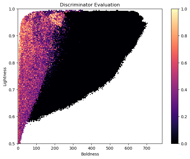
Now, we can plot a heatmap of the archive with the discriminator score. The large regions of low score (in black) show that many images in the archive are not realistic, even though LeNet-5 had high confidence that these images showed the digit eight.
plt.figure(figsize=(8, 6))
grid_archive_heatmap(discriminator_archive, vmin=0.0, vmax=1.0)
plt.title("Discriminator Evaluation")
plt.xlabel("Boldness")
plt.ylabel("Lightness")
plt.show()
Conclusion
By searching the latent space of an MNIST GAN, CMA-ME found images of the digit eight that varied in boldness and lightness. Even though the LeNet-5 network had high confidence that these images were eights, it turned out that many of these images were highly unrealistic, given that when we evaluated them with the GAN’s discriminator network, the images mostly received low scores.
In short, we found that large portions of the GAN’s latent space are unrealistic. This is not surprising because during training, the GAN generates fake images by randomly sampling the latent space from a fixed Gaussian distribution, and some portions of the distribution are less likely to be sampled. Thus, we have the following questions, which we leave open for future exploration:
How can we ensure that CMA-ME searches for realistic eights?
While searching for realistic eights, can we also search for other digits at the same time?
Citation
If you find this tutorial useful, please cite it as:
@article{pyribs_lsi_mnist,
  title   = {Illuminating the Latent Space of an MNIST GAN},
  author  = {Yulun Zhang and Bryon Tjanaka and Matthew C. Fontaine and Stefanos Nikolaidis},
  journal = {pyribs.org},
  year    = {2021},
  url     = {https://docs.pyribs.org/en/stable/tutorials/lsi_mnist.html}
}