ribs.visualize.grid_archive_heatmap¶

Plots heatmap of a GridArchive with 1D or 2D measure space.

This function creates a grid of cells and shades each cell with a color corresponding to the objective value of that cell’s elite. This function uses pcolormesh() to generate the grid. For further customization, pass extra kwargs to pcolormesh() through the pcm_kwargs parameter. For instance, to create black boundaries of width 0.1, pass in pcm_kwargs={"edgecolor": "black", "linewidth": 0.1}.

Examples

Heatmap of a 2D GridArchive

>>> import numpy as np
>>> import matplotlib.pyplot as plt
>>> from ribs.archives import GridArchive
>>> from ribs.visualize import grid_archive_heatmap
>>> # Populate the archive with the negative sphere function.
>>> archive = GridArchive(solution_dim=2,
...                       dims=[20, 20],
...                       ranges=[(-1, 1), (-1, 1)])
>>> x = np.random.uniform(-1, 1, 10000)
>>> y = np.random.uniform(-1, 1, 10000)
>>> archive.add(solution=np.stack((x, y), axis=1),
...             objective=-(x**2 + y**2),
...             measures=np.stack((x, y), axis=1))
>>> # Plot a heatmap of the archive.
>>> plt.figure(figsize=(8, 6))
>>> grid_archive_heatmap(archive)
>>> plt.title("Negative sphere function")
>>> plt.xlabel("x coords")
>>> plt.ylabel("y coords")
>>> plt.show()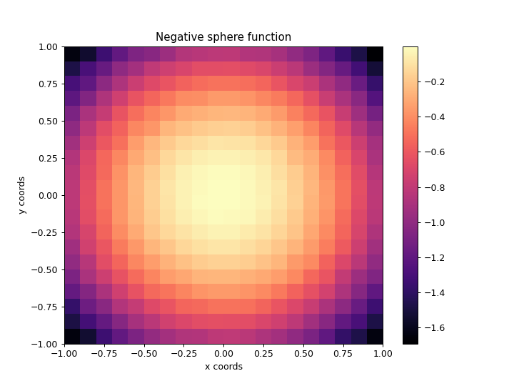

../_images/ribs-visualize-grid_archive_heatmap-1.png

Heatmap of a 1D GridArchive

>>> import numpy as np
>>> import matplotlib.pyplot as plt
>>> from ribs.archives import GridArchive
>>> from ribs.visualize import grid_archive_heatmap
>>> # Populate the archive with the negative sphere function.
>>> archive = GridArchive(solution_dim=2,
...                       dims=[20], ranges=[(-1, 1)])
>>> x = np.random.uniform(-1, 1, 1000)
>>> archive.add(solution=np.stack((x, x), axis=1),
...             objective=-x**2,
...             measures=x[:, None])
>>> # Plot a heatmap of the archive.
>>> plt.figure(figsize=(8, 6))
>>> grid_archive_heatmap(archive)
>>> plt.title("Negative sphere function with 1D measures")
>>> plt.xlabel("x coords")
>>> plt.show()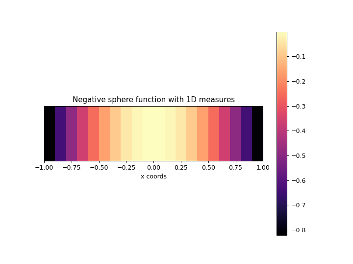

../_images/ribs-visualize-grid_archive_heatmap-2.png

Parameters:¶

archive: GridArchive¶: A 1D or 2D GridArchive.
ax: Axes | None = None¶: Axes on which to plot the heatmap. If None, the current axis will be used.
df: DataFrame | ArchiveDataFrame | None = None¶: If provided, we will plot data from this argument instead of the data currently in the archive. This data can be obtained by, for instance, calling ribs.archives.ArchiveBase.data() with return_type="pandas" and modifying the resulting ArchiveDataFrame. Note that, at a minimum, the data must contain columns for index, objective, and measures. To display a custom metric, replace the “objective” column.
transpose_measures: bool = False¶: By default, the first measure in the archive will appear along the x-axis, and the second will be along the y-axis. To switch this behavior (i.e. to transpose the axes), set this to True. Does not apply for 1D archives.
cmap: str | Sequence[matplotlib.typing.ColorType] | Colormap = 'magma'¶: The colormap to use when plotting intensity. Either the name of a Colormap, a list of Matplotlib color specifications (e.g., an \(N \times 3\) or \(N \times 4\) array – see ListedColormap), or a Colormap object.
aspect: 'auto' | 'equal' | float | None = None¶: The aspect ratio of the heatmap (i.e. height/width). Defaults to 'auto' for 2D and 0.5 for 1D. 'equal' is the same as aspect=1. See matplotlib.axes.Axes.set_aspect() for more info.
vmin: float | None = None¶: Minimum objective value to use in the plot. If None, the minimum objective value in the archive is used.
vmax: float | None = None¶: Maximum objective value to use in the plot. If None, the maximum objective value in the archive is used.
cbar: 'auto' | None | Axes = 'auto'¶: By default, this is set to 'auto' which displays the colorbar on the archive’s current Axes. If None, then colorbar is not displayed. If this is an Axes, displays the colorbar on the specified Axes.
cbar_kwargs: dict | None = None¶: Additional kwargs to pass to colorbar().
rasterized: bool = False¶: Whether to rasterize the heatmap. This can be useful for saving to a vector format like PDF. Essentially, only the heatmap will be converted to a raster graphic so that the archive cells will not have to be individually rendered. Meanwhile, the surrounding axes, particularly text labels, will remain in vector format.
pcm_kwargs: dict | None = None¶: Additional kwargs to pass to pcolormesh().

Raises:¶

ValueError – The archive’s measure dimension must be 1D or 2D.