ribs.visualize.cvt_archive_3d_plot¶

ribs.visualize.cvt_archive_3d_plot(archive: CVTArchive, ax: Axes3D | None = None, *, df: DataFrame | ArchiveDataFrame | None = None, measure_order: Iterable[int] | None = None, cmap: str | Sequence[matplotlib.typing.ColorType] | Colormap = 'magma', lw: float = 0.5, ec: matplotlib.typing.ColorType = (0.0, 0.0, 0.0, 0.1), cell_alpha: float = 1.0, vmin: float | None = None, vmax: float | None = None, cbar: 'auto' | None | Axes = 'auto', cbar_kwargs: dict | None = None, plot_elites: bool = False, elite_ms: float = 100, elite_alpha: float = 0.5, plot_centroids: bool = False, ms: float = 1, plot_samples: None = None) → None[source]¶

Plots a CVTArchive with 3D measure space.

This function relies on Matplotlib’s mplot3d toolkit. By default, this function plots a 3D Voronoi diagram of the cells in the archive and shades each cell based on its objective value. It is also possible to plot a “wireframe” with only the cells’ boundaries, along with a dot inside each cell indicating its objective value.

Depending on how many cells are in the archive, ms and lw may need to be tuned. If there are too many cells, the Voronoi diagram and centroid markers will make the entire image appear black. In that case, try turning off the centroids with plot_centroids=False or even removing the lines completely with lw=0.

Examples

3D Plot with Solid Cells

>>> import numpy as np
>>> import matplotlib.pyplot as plt
>>> from ribs.archives import CVTArchive
>>> from ribs.visualize import cvt_archive_3d_plot
>>> # Populate the archive with the negative sphere function.
>>> archive = CVTArchive(solution_dim=2,
...                      centroids=500,
...                      ranges=[(-2, 0), (-2, 0), (-2, 0)])
>>> x = np.random.uniform(-2, 0, 5000)
>>> y = np.random.uniform(-2, 0, 5000)
>>> z = np.random.uniform(-2, 0, 5000)
>>> archive.add(solution=np.stack((x, y), axis=1),
...             objective=-(x**2 + y**2 + z**2),
...             measures=np.stack((x, y, z), axis=1))
>>> # Plot the archive.
>>> plt.figure(figsize=(8, 6))
>>> cvt_archive_3d_plot(archive)
>>> plt.title("Negative sphere function with 3D measures")
>>> plt.show()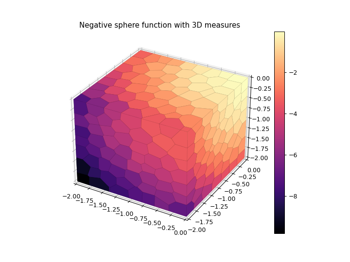

../_images/ribs-visualize-cvt_archive_3d_plot-1.png

3D Plot with Translucent Cells

>>> import numpy as np
>>> import matplotlib.pyplot as plt
>>> from ribs.archives import CVTArchive
>>> from ribs.visualize import cvt_archive_3d_plot
>>> # Populate the archive with the negative sphere function.
>>> archive = CVTArchive(solution_dim=2,
...                      centroids=500,
...                      ranges=[(-2, 0), (-2, 0), (-2, 0)])
>>> x = np.random.uniform(-2, 0, 5000)
>>> y = np.random.uniform(-2, 0, 5000)
>>> z = np.random.uniform(-2, 0, 5000)
>>> archive.add(solution=np.stack((x, y), axis=1),
...             objective=-(x**2 + y**2 + z**2),
...             measures=np.stack((x, y, z), axis=1))
>>> # Plot the archive.
>>> plt.figure(figsize=(8, 6))
>>> cvt_archive_3d_plot(archive, cell_alpha=0.1)
>>> plt.title("Negative sphere function with 3D measures")
>>> plt.show()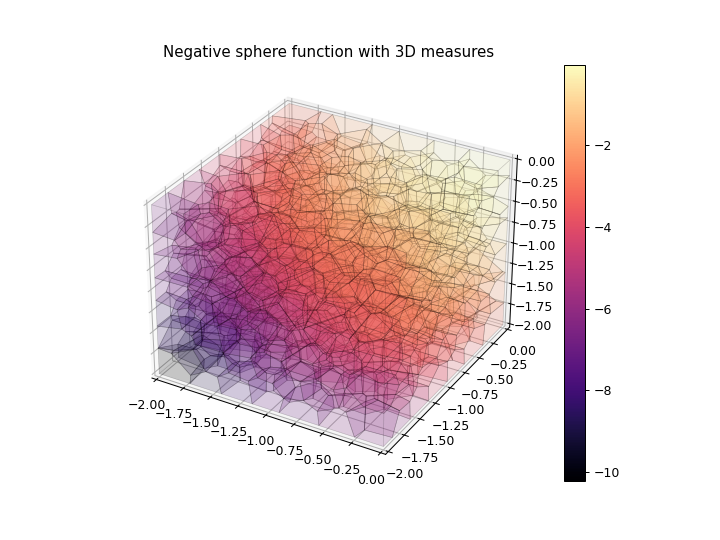

../_images/ribs-visualize-cvt_archive_3d_plot-2.png

3D “Wireframe” (Shading Turned Off)

>>> import numpy as np
>>> import matplotlib.pyplot as plt
>>> from ribs.archives import CVTArchive
>>> from ribs.visualize import cvt_archive_3d_plot
>>> # Populate the archive with the negative sphere function.
>>> archive = CVTArchive(solution_dim=2,
...                      centroids=100,
...                      ranges=[(-2, 0), (-2, 0), (-2, 0)])
>>> x = np.random.uniform(-2, 0, 1000)
>>> y = np.random.uniform(-2, 0, 1000)
>>> z = np.random.uniform(-2, 0, 1000)
>>> archive.add(solution=np.stack((x, y), axis=1),
...             objective=-(x**2 + y**2 + z**2),
...             measures=np.stack((x, y, z), axis=1))
>>> # Plot the archive.
>>> plt.figure(figsize=(8, 6))
>>> cvt_archive_3d_plot(archive, cell_alpha=0.0)
>>> plt.title("Negative sphere function with 3D measures")
>>> plt.show()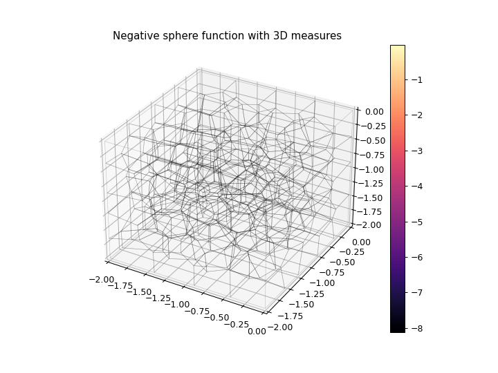

../_images/ribs-visualize-cvt_archive_3d_plot-3.png

3D Wireframe with Elites as Scatter Plot

>>> import numpy as np
>>> import matplotlib.pyplot as plt
>>> from ribs.archives import CVTArchive
>>> from ribs.visualize import cvt_archive_3d_plot
>>> # Populate the archive with the negative sphere function.
>>> archive = CVTArchive(solution_dim=2,
...                      centroids=100,
...                      ranges=[(-2, 0), (-2, 0), (-2, 0)])
>>> x = np.random.uniform(-2, 0, 1000)
>>> y = np.random.uniform(-2, 0, 1000)
>>> z = np.random.uniform(-2, 0, 1000)
>>> archive.add(solution=np.stack((x, y), axis=1),
...             objective=-(x**2 + y**2 + z**2),
...             measures=np.stack((x, y, z), axis=1))
>>> # Plot the archive.
>>> plt.figure(figsize=(8, 6))
>>> cvt_archive_3d_plot(archive, cell_alpha=0.0, plot_elites=True)
>>> plt.title("Negative sphere function with 3D measures")
>>> plt.show()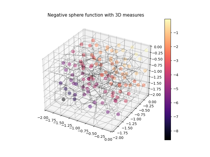

../_images/ribs-visualize-cvt_archive_3d_plot-4.png

Parameters:¶

archive: CVTArchive¶: A 3D CVTArchive.
ax: Axes3D | None = None¶: Axes on which to plot the heatmap. If None, we will create a new 3D axis.
df: DataFrame | ArchiveDataFrame | None = None¶: If provided, we will plot data from this argument instead of the data currently in the archive. This data can be obtained by, for instance, calling ribs.archives.ArchiveBase.data() with return_type="pandas" and modifying the resulting ArchiveDataFrame. Note that, at a minimum, the data must contain columns for index, objective, and measures. To display a custom metric, replace the “objective” column.
measure_order: Iterable[int] | None = None¶: Specifies the axes order for plotting the measures. By default, the first measure (measure 0) in the archive appears on the x-axis, the second (measure 1) on y-axis, and third (measure 2) on z-axis. This argument is an array of length 3 that specifies which measure should appear on the x, y, and z axes. For instance, [2, 1, 0] will put measure 2 on the x-axis, measure 1 on the y-axis, and measure 0 on the z-axis.
cmap: str | Sequence[matplotlib.typing.ColorType] | Colormap = 'magma'¶: The colormap to use when plotting intensity. Either the name of a Colormap, a list of Matplotlib color specifications (e.g., an \(N \times 3\) or \(N \times 4\) array – see ListedColormap), or a Colormap object.
lw: float = 0.5¶: Line width when plotting the Voronoi diagram.
ec: matplotlib.typing.ColorType = (0.0, 0.0, 0.0, 0.1)¶: Edge color of the cells in the Voronoi diagram. See here for more info on specifying colors in Matplotlib.
cell_alpha: float = 1.0¶: Alpha value for the cell colors. Set to 1.0 for opaque cells; set to 0.0 for fully transparent cells.
vmin: float | None = None¶: Minimum objective value to use in the plot. If None, the minimum objective value in the archive is used.
vmax: float | None = None¶: Maximum objective value to use in the plot. If None, the maximum objective value in the archive is used.
cbar: 'auto' | None | Axes = 'auto'¶: By default, this is set to 'auto' which displays the colorbar on the archive’s current Axes. If None, then colorbar is not displayed. If this is an Axes, displays the colorbar on the specified Axes.
cbar_kwargs: dict | None = None¶: Additional kwargs to pass to colorbar().
plot_elites: bool = False¶: If True, we will plot a scatter plot of the elites in the archive. The elites will be colored according to their objective value.
elite_ms: float = 100¶: Marker size for plotting elites.
elite_alpha: float = 0.5¶: Alpha value for plotting elites.
plot_centroids: bool = False¶: Whether to plot the cluster centroids.
ms: float = 1¶: Marker size for centroids.
plot_samples: None = None¶: DEPRECATED.

Raises:¶

ValueError – The archive’s measure dimension must be 1D or 2D.
ValueError – measure_order is not a permutation of [0, 1, 2].