ribs.visualize.archive_histogram¶

Plots a histogram of the objective values in an archive.

In short, this function is a wrapper around Matplotlib’s hist(). It calls hist with objective values retrieved from the archive and then applies a number of (opinionated) customizations. As such, many of this function’s arguments are shared with hist.

Note

This function is intended to plot a single archive, similar to heatmap functions. To aggregate multiple archives into a CDF/CCDF or histogram, see aggregate_cdf().

Examples

Basic Histogram of a 2D GridArchive

import numpy as np
import matplotlib.pyplot as plt
from ribs.archives import GridArchive
from ribs.visualize import archive_histogram

# Populate the archive with the negative sphere function.
archive = GridArchive(solution_dim=2,
                      dims=[100, 100],
                      ranges=[(-1, 1), (-1, 1)])
x = np.random.uniform(-1, 1, 10000)
y = np.random.uniform(-1, 1, 10000)
archive.add(solution=np.stack((x, y), axis=1),
            objective=-(x**2 + y**2),
            measures=np.stack((x, y), axis=1))

# Plot a histogram of the archive.
plt.figure(figsize=(8, 6))
archive_histogram(archive)
plt.xlabel("Objective")
plt.ylabel("Num. Elites")
plt.show()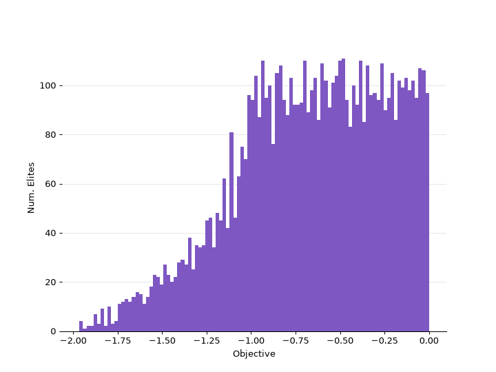

../_images/ribs-visualize-archive_histogram-1.png

Histogram Where Bars Are Colored With a Colormap

import numpy as np
import matplotlib.pyplot as plt
from ribs.archives import GridArchive
from ribs.visualize import archive_histogram

# Populate the archive with the negative sphere function.
archive = GridArchive(solution_dim=2,
                      dims=[100, 100],
                      ranges=[(-1, 1), (-1, 1)])
x = np.random.uniform(-1, 1, 10000)
y = np.random.uniform(-1, 1, 10000)
archive.add(solution=np.stack((x, y), axis=1),
            objective=-(x**2 + y**2),
            measures=np.stack((x, y), axis=1))

# Plot a histogram of the archive.
plt.figure(figsize=(8, 6))
archive_histogram(archive, cmap="magma")
plt.xlabel("Objective")
plt.ylabel("Num. Elites")
plt.show()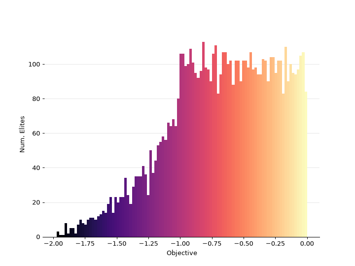

../_images/ribs-visualize-archive_histogram-2.png

Histogram with More Customizations

import numpy as np
import matplotlib.pyplot as plt
from ribs.archives import GridArchive
from ribs.visualize import archive_histogram

# Populate the archive with the negative sphere function.
archive = GridArchive(solution_dim=2,
                      dims=[100, 100],
                      ranges=[(-1, 1), (-1, 1)])
x = np.random.uniform(-1, 1, 10000)
y = np.random.uniform(-1, 1, 10000)
archive.add(solution=np.stack((x, y), axis=1),
            objective=-(x**2 + y**2),
            measures=np.stack((x, y), axis=1))

# Plot a histogram of the archive.
plt.figure(figsize=(8, 6))
archive_histogram(
    archive,
    bins=50,  # Only use 50 bins.
    vmin=-2.5,  # Minimum objective value.
    vmax=0.5,  # Maximum objective value.
    ylim=400,  # Set the top of the y-axis.
)
plt.xlabel("Objective")
plt.ylabel("Num. Elites")
plt.show()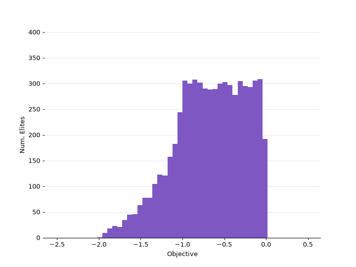

../_images/ribs-visualize-archive_histogram-3.png

Parameters:¶

archive: ArchiveBase¶: An archive that can provide its objective values via the data() method.
ax: Axes | None = None¶: Axes on which to plot the histogram. If None, the current axis will be used.
df: DataFrame | ArchiveDataFrame | None = None¶: If provided, we will plot data from this argument instead of the data currently in the archive. This data can be obtained by, for instance, calling ribs.archives.ArchiveBase.data() with return_type="pandas" and modifying the resulting ArchiveDataFrame. Note that, at a minimum, the data must contain a column for “objective”.
bins: int | Sequence[float] | str | None = 100¶: Bins for the histogram. The default of 100 indicates that the histogram will consist of 100 equally-sized bins. See hist() for more info.
vmin: float | None = None¶: Minimum objective value to use in the plot. If None, the minimum objective value in the archive is used.
vmax: float | None = None¶: Maximum objective value to use in the plot. If None, the maximum objective value in the archive is used.
ylim: float | None = None¶: If provided, this is used to set the top ylimit (i.e., the upper bound of the y-axis) for the histogram.
color: matplotlib.typing.ColorType = '#7e57c2'¶: Color of the histogram bars. Defaults to the pyribs theme color. Refer to this Matplotlib page for more info on specifying colors.
cmap: str | Sequence[matplotlib.typing.ColorType] | Colormap | None = None¶: Instead of passing in color, a colormap can be passed in to color the histogram bars according to their objective value. This parameter can either be the name of a Colormap, a list of Matplotlib color specifications (e.g., an \(N \times 3\) or \(N \times 4\) array – see ListedColormap), or a Colormap object. For example, “magma” is the default used in the Pyribs heatmap visualizations. If both color and cmap are passed in, the cmap will take precedence.
rasterized: bool = False¶: Whether to rasterize the bars of the histogram. This can be useful for saving to a vector format like PDF. Essentially, only the bars will be converted to a raster graphic, so that they will not have to be individually rendered. Meanwhile, the surrounding axes, particularly text labels, will remain in vector format.
hist_kwargs: dict | None = None¶: Additional kwargs to pass to hist(). Note that since hist calls numpy.histogram(), some of these arguments may ultimately go to histogram. Note that we already pass the following parameters: bins, range (via vmin and vmax), color, and rasterized.

Raises:¶

AttributeError – The data() method is not implemented on the given archive, which prevents retrieving its objective values.