Using CMA-ME to Land a Lunar Lander Like a Space Shuttle
![]()
This tutorial is part of the series of pyribs tutorials! See here for the list of all tutorials and the order in which they should be read.
In the Lunar Lander environment, an agent controls a spaceship to touch down gently within a goal zone near the bottom of the screen. Typically, agents in Lunar Lander take a direct approach, hovering straight down:
from __future__ import annotations

from IPython.display import HTML, display  # noqa: A004

display(HTML("""<video width="360" height="auto" controls><source src="https://raw.githubusercontent.com/icaros-usc/pyribs/master/docs/_static/imgs/lunar-lander-vertical.mp4" type="video/mp4" /></video>"""))  # fmt: skip
Of course, this works fine, and the lander safely lands on the landing pad. However, there are many (and more theatric) ways we can safely achieve our goal. For instance, a different solution is to land like a space shuttle:
display(HTML("""<video width="360" height="auto" controls><source src="https://raw.githubusercontent.com/icaros-usc/pyribs/master/docs/_static/imgs/lunar-lander-left.mp4" type="video/mp4" /></video>""")) # fmt: skip
And we can also approach from the right:
display(HTML("""<video width="360" height="auto" controls><source src="https://raw.githubusercontent.com/icaros-usc/pyribs/master/docs/_static/imgs/lunar-lander-right.mp4" type="video/mp4" /></video>""")) # fmt: skip
The primary difference between these trajectories is their “point of impact,” that is, the \(x\)-position of the lander when one of its legs hits the ground for the first time. In the vertical trajectory, the lander first impacts the ground at \(x \approx -0.1\), and when approaching from the left and right, it first impacts at \(x \approx -0.5\) and \(x \approx 0.6\), respectively.
Though these trajectories look different, they all achieve good performance (200+), leading to an important insight: there are characteristics of landing a lunar lander that are not necessarily important for performance, but nonetheless determine the behavior of the lander. In quality diversity (QD) terms, we call these measures. In this tutorial, we will search for policies that yield different trajectories using the pyribs implementation of the QD algorithm CMA-ME.
By the way: Recent work introduced CMA-MAE, an algorithm which builds on CMA-ME and achieves higher performance in a variety of domains. Once you finish this tutorial, be sure to check out the next tutorial to learn about CMA-MAE.
Setup
First, let’s install pyribs and Gymnasium. Gymnasium is the successor to OpenAI Gym, which was deprecated in late 2022. We use the visualize extra of pyribs (ribs[visualize] instead of just ribs) so that we obtain access to the ribs.visualize module.
%pip install swig  # Must be installed before box2d.
%pip install ribs[visualize] tqdm "gymnasium[box2d]>=1.0.0" "moviepy>=1.0.0" dask distributed
Now, we import Gymnasium and several utilities.
import sys
import time

import gymnasium as gym
import matplotlib.pyplot as plt
import numpy as np
from dask.distributed import Client
from tqdm import tqdm, trange
Problem Description
We treat the Lunar Lander as a quality diversity (QD) problem. For the objective, we use the default rewards provided by the environment, which encourages landing on the landing pad and penalizes engine usage.
For the measure functions, we are interested in several factors at the time of “impact.” We define impact to be the first time when either of the lunar lander’s legs touches the ground. When this happens, we measure the following:
\(x\)-position: This will lead to markedly different trajectories, as seen earlier.
\(y\)-velocity: Different velocities will determine how hard the lander impacts the ground.
If the lunar lander never impacts the ground, we default the \(x\)-position to be the last \(x\)-position of the lander, and the \(y\)-velocity to be the maximum velocity of the lander (technically minimum since velocities are negative).
We will search for policies that produce high-performing trajectories with these measures. For simplicity, we will use a linear policy to control the lunar lander. As the default lunar lander has discrete controls, the equation for this policy is:
where \(a\) is the action to take, \(s\) is the state vector, and \(W\) is our model, a matrix of weights that stays constant. Essentially, we transform the state to a vector with a “signal” for each possible action in the action space, and we choose the action with the highest signal. To search for a different policy, we explore the space of models \(W\).
In this tutorial, we will search for policies solving a fixed scenario with a flat terrain. To create this scenario, we use a fixed seed of 52 in the environment.
Note: Determinism
Since our policy and environment are both deterministic, we only have to simulate the policy once to find its performance. Typically, we would run our policy multiple times to gauge average performance and have it generalize, but we ignore that to keep this example simple.
# Create an environment so that we can obtain information about it.
reference_env = gym.make("LunarLander-v3")
action_dim = reference_env.action_space.n
obs_dim = reference_env.observation_space.shape[0]

# Seed for all environments in this notebook.
env_seed = 52
We can summarize our problem description with the following simulate function, which takes in the model and rolls it out in the Lunar Lander environment.
def simulate(
    model: np.ndarray, seed: int | None = None, video_env: gym.Env | None = None
) -> tuple[float, float, float]:
    """Simulates the lunar lander model.

    Args:
        model: The array of weights for the linear policy.
        seed: The seed for the environment.
        video_env: If passed in, this will be used instead of creating a new env. This
            is used primarily for recording video during evaluation.

    Returns:
        total_reward: The reward accrued by the lander throughout its trajectory.
        impact_x_pos: The x position of the lander when it touches the ground for the
            first time.
        impact_y_vel: The y velocity of the lander when it touches the ground for the
            first time.
    """
    if video_env is None:
        # Since we are using multiple processes, it is simpler if each worker just
        # creates their own copy of the environment instead of trying to share the
        # environment. This also makes the function "pure." However, we should use the
        # video_env if it is passed in.
        env = gym.make("LunarLander-v3")
    else:
        env = video_env

    action_dim = env.action_space.n
    obs_dim = env.observation_space.shape[0]
    model = model.reshape((action_dim, obs_dim))

    total_reward = 0.0
    impact_x_pos = None
    impact_y_vel = None
    all_y_vels = []
    obs, _ = env.reset(seed=seed)
    done = False

    while not done:
        action = np.argmax(model @ obs)  # Linear policy.
        obs, reward, terminated, truncated, _ = env.step(action)
        done = terminated or truncated
        total_reward += reward

        # Refer to the definition of state here:
        # https://gymnasium.farama.org/environments/box2d/lunar_lander/
        x_pos = obs[0]
        y_vel = obs[3]
        leg0_touch = bool(obs[6])
        leg1_touch = bool(obs[7])
        all_y_vels.append(y_vel)

        # Check if the lunar lander is impacting for the first time.
        if impact_x_pos is None and (leg0_touch or leg1_touch):
            impact_x_pos = x_pos
            impact_y_vel = y_vel

    # If the lunar lander did not land, set the x-pos to the one from the final
    # timestep, and set the y-vel to the max y-vel (we use min since the lander goes
    # down).
    if impact_x_pos is None:
        impact_x_pos = x_pos
        impact_y_vel = min(all_y_vels)

    # Only close the env if it was not a video env.
    if video_env is None:
        env.close()

    return total_reward, impact_x_pos, impact_y_vel
CMA-ME with pyribs
To train our policy, we will use the CMA-ME algorithm (if you are not familiar with CMA-ME, please refer to the corresponding paper). This means we need to import and initialize the GridArchive, EvolutionStrategyEmitter, and Scheduler from pyribs.
GridArchive
First, the GridArchive stores solutions (i.e. models for our policy) in a rectangular grid. Each dimension of the GridArchive corresponds to a dimension in measure space that is segmented into equally sized cells. As we have two measure functions for our lunar lander, we have two dimensions in the GridArchive. The first dimension is the impact \(x\)-position, which ranges from -1 to 1, and the second is the impact \(y\)-velocity, which ranges from -3 (smashing into the ground) to 0 (gently touching down). We divide both dimensions into 50 cells.
We additionally specify the dimensionality of solutions which will be stored in the archive. While each model is a 2D matrix, pyribs archives only allow 1D arrays for efficiency; hence, we create an initial_model below and retrieve the size of its flattened, 1D form with initial_model.size.
from ribs.archives import GridArchive

initial_model = np.zeros((action_dim, obs_dim))

archive = GridArchive(
    solution_dim=initial_model.size,  # Dimensionality of solutions in the archive.
    dims=[50, 50],  # 50 cells along each dimension.
    ranges=[(-1.0, 1.0), (-3.0, 0.0)],  # (-1, 1) for x-pos and (-3, 0) for y-vel.
    qd_score_offset=-600,  # See the note below.
)
Note: QD Score Offset
Above, we specified
qd_score_offset=-600when initializing the archive. The QD score (Pugh 2016) is a metric for QD algorithms which sums the objective values of all elites in the archive. However, if objectives can be negative, this metric will penalize an algorithm for discovering new cells with a negative objective. To prevent this, it is common to normalize each objective to be non-negative by subtracting an offset, typically the minimum objective, before computing the QD score. While lunar lander does not have a predefined minimum objective, we know from previous experiments that almost all solutions score above -600, so we have set the offset accordingly. Thus, if a solution has, for example, an objective of -300, then its objective will be normalized to -300 - (-600) = 300.
Note: Keyword Arguments
In pyribs, most constructor arguments must be keyword arguments. For example, the
GridArchiveconstructor looks likeGridArchive(*, solution_dim, ...). Notice the*in the parameter list. This*syntax indicates that any parameters listed after it must be passed as keyword arguments, e.g.,GridArchive(solution_dim=initial_model.size, ...)as is done above. Furthermore, passing a positional argument likeGridArchive(10, ...)would throw aTypeError. We adopt this practice from scikit-learn in an effort to increase code readability.
EvolutionStrategyEmitter
Next, the EvolutionStrategyEmitter with two-stage improvement ranking (“2imp”) uses CMA-ES to search for policies that add new entries to the archive or improve existing ones. Since we do not have any prior knowledge of what the model will be, we set the initial model to be the zero vector, and we set the initial step size for CMA-ES to be 1.0, so that initial solutions are sampled from a standard isotropic Gaussian. Furthermore, we use 5 emitters so that the algorithm simultaneously searches several areas of the measure space.
from ribs.emitters import EvolutionStrategyEmitter

emitters = [
    EvolutionStrategyEmitter(
        archive=archive,
        x0=initial_model.flatten(),
        sigma0=1.0,  # Initial step size.
        ranker="2imp",
        # If we do not specify a batch size, the emitter will automatically use a
        # batch size equal to the default population size of CMA-ES.
        batch_size=30,
    )
    for _ in range(5)  # Create 5 separate emitters.
]
Note: Two-Stage Improvement Ranking
The term “two-stage” refers to how this ranking mechanism ranks solutions by a tuple of
(status, value)defined as follows:
status: Whether the solution creates a new cell in the archive, improves an existing cell, or is not inserted.
value: Consider the objective \(f\) of the solution and the objective \(f'\) of the solution currently in the cell where the solution will be inserted. When the solution creates a new cell, \(f'\) is undefined because the cell was previously empty, so the value is defined as \(f\). Otherwise, when the solution improves an existing cell or is not inserted at all, the value is \(f - f'\).During ranking, this two-stage improvement ranker will first sort by
status, prioritizing new solutions, followed by solutions which improve existing cells, followed by solutions which are not inserted. Within each group, solutions are further ranked by their correspondingvalue. See the archiveaddmethod for more information on statuses and values.Additional rankers are available in the ribs.emitters.rankers module. These rankers include those corresponding to different emitters described in the CMA-ME paper.
Scheduler
Finally, the Scheduler controls how the emitters interact with the archive. On every iteration, the scheduler calls the emitters to generate solutions. After the user evaluates these generated solutions, the scheduler inserts the solutions into the archive and passes the feedback to the emitters (this feedback consists of the status and value for each solution that we described in the note above).
from ribs.schedulers import Scheduler

scheduler = Scheduler(archive, emitters)
QD Search
With the pyribs components defined, we start searching with CMA-ME. Since we use 5 emitters each with a batch size of 30 and we run 300 iterations, we run 5 x 30 x 300 = 45,000 lunar lander simulations. We also keep track of some logging info via archive.stats, which is an ArchiveStats object.
Since it takes a relatively long time to evaluate a lunar lander solution, we parallelize the evaluation of multiple solutions with Dask. On Colab, with one worker (i.e., one CPU), the loop should take ~30 minutes to run. With two workers, it should take ~20 minutes to run. Feel free to increase the number of workers based on the number of CPUs your system has available to speed up the loop further.
start_time = time.time()
total_itrs = 300
workers = 2  # Adjust the number of workers based on your available CPUs.

client = Client(
    n_workers=workers,  # Create this many worker processes using Dask LocalCluster.
    threads_per_worker=1,  # Each worker process is single-threaded.
)

for itr in trange(1, total_itrs + 1, file=sys.stdout, desc="Iterations"):
    # Request models from the scheduler.
    solutions = scheduler.ask()

    # Evaluate the models and record the objectives and measuress.
    futures = client.map(lambda model: simulate(model, env_seed), solutions)
    results = client.gather(futures)

    objectives, measures = [], []
    for obj, impact_x_pos, impact_y_vel in results:
        objectives.append(obj)
        measures.append([impact_x_pos, impact_y_vel])

    # Send the results back to the scheduler.
    scheduler.tell(objectives, measures)

    # Logging.
    if itr % 25 == 0 or itr == total_itrs:
        # fmt: off
        tqdm.write(f"> {itr} itrs completed after {time.time() - start_time:.2f}s")
        tqdm.write(f"  - Size: {archive.stats.num_elites}")    # Number of elites in the archive. len(archive) also provides this info.
        tqdm.write(f"  - Coverage: {archive.stats.coverage}")  # Proportion of archive cells which have an elite.
        tqdm.write(f"  - QD Score: {archive.stats.qd_score}")  # QD score, i.e. sum of objective values of all elites in the archive.
                                                               # Accounts for qd_score_offset as described in the GridArchive section.
        tqdm.write(f"  - Max Obj: {archive.stats.obj_max}")    # Maximum objective value in the archive.
        tqdm.write(f"  - Mean Obj: {archive.stats.obj_mean}")  # Mean objective value of elites in the archive.
        # fmt: on
> 25 itrs completed after 27.07s
  - Size: 1085
  - Coverage: 0.434
  - QD Score: 497644.71204478183
  - Max Obj: 309.7382675521822
  - Mean Obj: -141.34127922139925
> 50 itrs completed after 55.04s
  - Size: 1673
  - Coverage: 0.6692
  - QD Score: 732461.1952852886
  - Max Obj: 309.7382675521822
  - Mean Obj: -162.18697233395778
> 75 itrs completed after 81.05s
  - Size: 2078
  - Coverage: 0.8312
  - QD Score: 861943.2417494163
  - Max Obj: 309.7382675521822
  - Mean Obj: -185.20536970672939
> 100 itrs completed after 112.97s
  - Size: 2332
  - Coverage: 0.9328
  - QD Score: 1017846.2654447029
  - Max Obj: 309.7382675521822
  - Mean Obj: -163.53076095853217
> 125 itrs completed after 140.89s
  - Size: 2399
  - Coverage: 0.9596
  - QD Score: 1125383.7911532177
  - Max Obj: 309.7382675521822
  - Mean Obj: -130.89462644717895
> 150 itrs completed after 175.00s
  - Size: 2457
  - Coverage: 0.9828
  - QD Score: 1211303.3135671858
  - Max Obj: 309.7382675521822
  - Mean Obj: -106.99905837721377
> 175 itrs completed after 216.63s
  - Size: 2476
  - Coverage: 0.9904
  - QD Score: 1262819.5040088487
  - Max Obj: 309.7382675521822
  - Mean Obj: -89.97596768624851
> 200 itrs completed after 253.28s
  - Size: 2482
  - Coverage: 0.9928
  - QD Score: 1299446.9768728297
  - Max Obj: 309.7382675521822
  - Mean Obj: -76.45166121159157
> 225 itrs completed after 289.28s
  - Size: 2486
  - Coverage: 0.9944
  - QD Score: 1327841.5868551808
  - Max Obj: 315.29614111938383
  - Mean Obj: -65.87224985712763
> 250 itrs completed after 317.58s
  - Size: 2493
  - Coverage: 0.9972
  - QD Score: 1347854.8429337537
  - Max Obj: 315.29614111938383
  - Mean Obj: -59.34422666114973
> 275 itrs completed after 347.03s
  - Size: 2495
  - Coverage: 0.998
  - QD Score: 1363806.922283271
  - Max Obj: 315.29614111938383
  - Mean Obj: -53.383999084861294
> 300 itrs completed after 375.14s
  - Size: 2497
  - Coverage: 0.9988
  - QD Score: 1374444.5067896002
  - Max Obj: 315.29614111938383
  - Mean Obj: -49.561671289707576
Iterations: 100%|████████████████████████████████████████| 300/300 [06:14<00:00,  1.25s/it]
Visualizing the Archive
Using grid_archive_heatmap from the ribs.visualize module, we can view a heatmap of the archive. The heatmap shows the measures for which CMA-ME found a solution. The color of each cell shows the objective value of the solution.
from ribs.visualize import grid_archive_heatmap

plt.figure(figsize=(8, 6))
grid_archive_heatmap(archive, vmin=-300, vmax=300)
plt.gca().invert_yaxis()  # Makes more sense if larger velocities are on top.
plt.ylabel("Impact y-velocity")
plt.xlabel("Impact x-position")
Text(0.5, 0, 'Impact x-position')
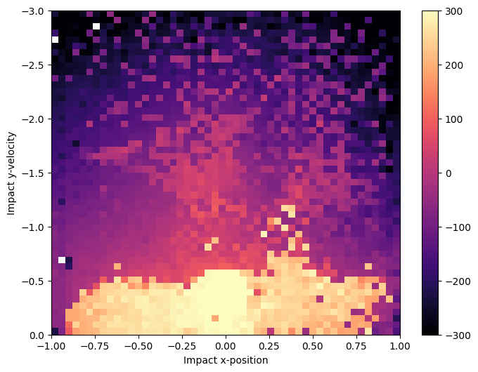
From this heatmap, we can make a few observations:
CMA-ME found solutions for almost all cells in the archive (empty cells show up as white).
Most of the high-performing solutions have lower impact \(y\)-velocities (see the bright area at the bottom of the map). This is reasonable, as a lander that crashes into the ground would not do well.
The high-performing solutions are spread across a wide range of impact \(x\)-positions. The highest solutions seem to be at \(x \approx 0\) (the bright spot in the middle). This makes sense since an impact \(x\)-position of 0 corresponds to the direct vertical approach. Nevertheless, there are many high-performing solutions that had other \(x\)-positions, and we will visualize them in the next section.
Visualizing Individual Trajectories
To view the trajectories for different models, we can use the RecordVideo wrapper, and we can use IPython to display the video in the notebook. The display_video function below shows how to do this.
import base64
import glob

from IPython.display import HTML, display  # noqa: A004


def display_video(model: np.ndarray) -> None:
    """Displays a video of the model in the environment."""
    video_env = gym.wrappers.RecordVideo(
        gym.make("LunarLander-v3", render_mode="rgb_array"),
        video_folder="videos",
        # This will ensure all episodes are recorded as videos.
        episode_trigger=lambda idx: True,  # noqa: ARG005
        # Disables moviepy's logger to reduce clutter in the output.
        disable_logger=True,
    )
    simulate(model, env_seed, video_env)
    video_env.close()  # Save video.

    # Display the video with HTML. Though we use glob, there is only 1 video.
    for video_path in glob.glob("videos/*.mp4"):
        with open(video_path, "rb") as video_file:
            video = video_file.read()
        encoded = base64.b64encode(video).decode("ascii")
        display(
            HTML(f"""
            <video width="360" height="auto" controls>
                <source src="data:video/mp4;base64,{encoded}" type="video/mp4" />
            </video>""")
        )
We can retrieve policies with measures that are close to a query with the retrieve_single method. This method will look up the cell corresponding to the queried measures. Then, the method will check if there is an elite in that cell, and return the elite if it exists (the method does not check neighboring cells for elites). The returned elite may not have the exact measures requested because the elite only has to be in the same cell as the queried measures.
Below, we first retrieve a policy that impacted the ground on the left (approximately -0.4) with low velocity (approximately -0.10) by querying for [-0.4, -0.10].
occupied, elite = archive.retrieve_single([-0.4, -0.10])
# `occupied` indicates if there was an elite in the corresponding cell.
if occupied:
    print(f"Objective: {elite['objective']}")
    print(f"Measures: (x-pos: {elite['measures'][0]}, y-vel: {elite['measures'][1]})")
    display_video(elite["solution"])
Objective: 271.3673071671791
Measures: (x-pos: -0.3962918221950531, y-vel: -0.09530427306890488)
We can also find a policy that impacted the ground on the right (0.6) with low velocity.
Note: Batch and Single Methods
retrieve_singlereturns an elite represented as a dict, given a singlemeasuresarray. Meanwhile, theretrievemethod takes in a batch ofmeasuresand returns a dict holding batches of data. Several archive methods in pyribs follow a similar pattern of having a batch and single version, e.g.,addandadd_single.
occupied, elite = archive.retrieve_single([0.6, -0.10])
if occupied:
    print(f"Objective: {elite['objective']}")
    print(f"Measures: (x-pos: {elite['measures'][0]}, y-vel: {elite['measures'][1]})")
    display_video(elite["solution"])
Objective: 194.52479264536845
Measures: (x-pos: 0.6237214803695679, y-vel: -0.07001425325870514)
And we can find a policy that executes a regular vertical landing, which happens when the impact \(x\)-position is around 0.
occupied, elite = archive.retrieve_single([0.0, -0.10])
if occupied:
    print(f"Objective: {elite['objective']}")
    print(f"Measures: (x-pos: {elite['measures'][0]}, y-vel: {elite['measures'][1]})")
    display_video(elite["solution"])
Objective: 306.5193835015769
Measures: (x-pos: 0.038937948644161224, y-vel: -0.07311394810676575)
As the archive has ~2500 solutions, we cannot view them all, but we can filter for high-performing solutions. We first retrieve the archive’s elites with the data method with return_type="pandas". Then, we choose solutions that scored above 200 because 200 is the threshold for the problem to be considered solved. Note that many high-performing solutions do not land on the landing pad.
df = archive.data(return_type="pandas")
high_perf_sols = df.query("objective > 200").sort_values("objective", ascending=False)
Below we visualize several of these high-performing solutions. The iterelites method is available because data returns an ArchiveDataFrame, a subclass of the Pandas DataFrame specialized for pyribs. iterelites iterates over the entries in the DataFrame and returns them as dicts.
if len(high_perf_sols) > 0:
    for elite in high_perf_sols.iloc[[0, len(high_perf_sols) // 2, -1]].iterelites():
        print(f"Objective: {elite['objective']}")
        print(
            f"Measures: (x-pos: {elite['measures'][0]}, y-vel: {elite['measures'][1]})"
        )
        display_video(elite["solution"])
Objective: 315.29614111938383
Measures: (x-pos: -0.028294086456298828, y-vel: -0.4220752716064453)
Objective: 255.2233471793768
Measures: (x-pos: 0.28050756454467773, y-vel: -0.4443489611148834)
Objective: 200.0387419424668
Measures: (x-pos: 0.3441486358642578, y-vel: -0.741992712020874)
And finally, the best_elite property is the elite that has the highest performance in the archive.
print(f"Objective: {archive.best_elite['objective']}")
print(
    f"Measures: (x-pos: {archive.best_elite['measures'][0]}, y-vel: {archive.best_elite['measures'][1]})"
)
display_video(archive.best_elite["solution"])
Objective: 315.29614111938383
Measures: (x-pos: -0.028294086456298828, y-vel: -0.4220752716064453)
Conclusion
As the saying goes, “there is more than one way to land an airplane” 😉. However, it is often difficult to shape the reward function in reinforcement learning to discover these unique and “creative” solutions. In such cases, a QD algorithm can help search for solutions that vary in “interestingness.”
In this tutorial, we showed that this is the case for the lunar lander environment. Using CMA-ME, we searched for lunar lander trajectories with differing impact measures. Though these trajectories all take a different approach, many perform well.
For extending this tutorial, we suggest the following:
Replace the impact measures with your own measures. What other properties might be interesting for the lunar lander?
Try different terrains by changing the seed. For instance, if the environment has valleys, can the lander learn to go into this valley and glide back up?
Try increasing the number of iterations. Will CMA-ME create a better archive if it gets to evaluate more solutions?
Use other gym environments. What measures could you use in an environment like
BipedalWalker-v2?
Finally, to learn about an algorithm which performs even better on QD problems, check out the CMA-MAE tutorial.
And for a version of this tutorial that uses Dask to parallelize evaluations and offers features like a command-line interface, refer to the Lunar Lander example.
Citation
If you find this tutorial useful, please cite it as:
@article{pyribs_lunar_lander,
  title   = {Using CMA-ME to Land a Lunar Lander Like a Space Shuttle},
  author  = {Bryon Tjanaka and Sam Sommerer and Nikitas Klapsis and Matthew C. Fontaine and Stefanos Nikolaidis},
  journal = {pyribs.org},
  year    = {2021},
  url     = {https://docs.pyribs.org/en/stable/tutorials/lunar_lander.html}
}
Credits
This tutorial is based on a poster created by Nikitas Klapsis as part of USC’s 2020 SHINE program.